EpistasisNonlinearRegression: two-stage fitting
Many biophysical phenotypes (fluorescence, growth rate, binding affinity) are measured on an inherently nonlinear scale. If you fit a linear epistasis model directly to such data, the recovered coefficients conflate genuine genetic interactions with the curvature of the measurement scale. EpistasisNonlinearRegression separates these effects with a two-stage procedure: it first learns an additive linear representation of the landscape, then fits a user-supplied nonlinear function that maps the additive phenotype to the observed measurement scale.

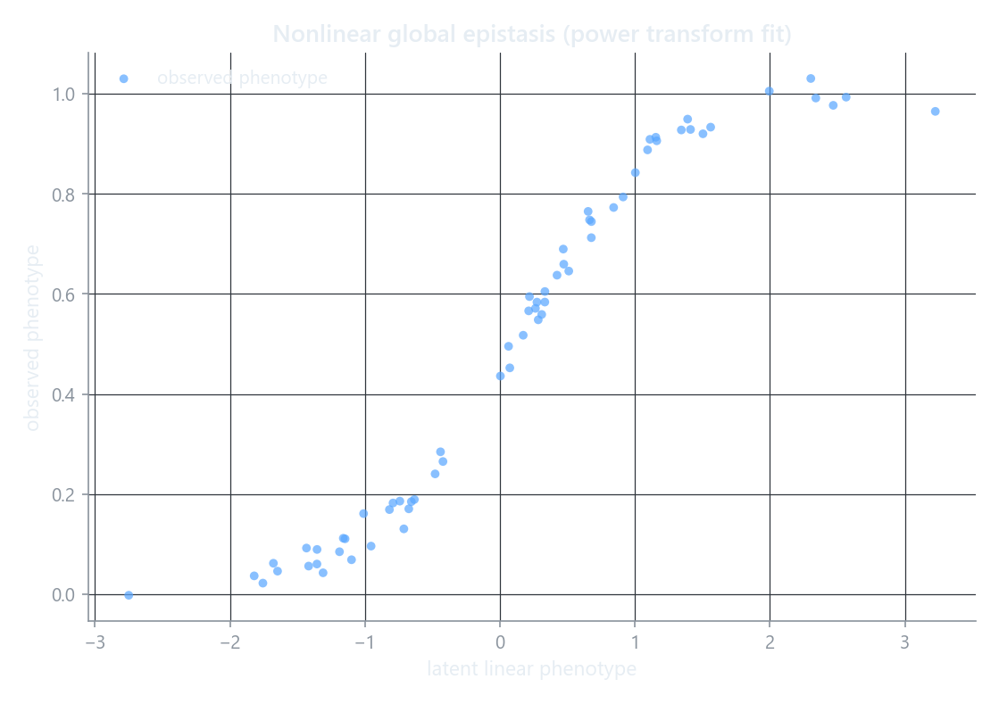
EpistasisPowerTransform (a Box-Cox-style scale, Sailer & Harms 2017) is the worked example above: the fitted curve is the nonlinear map from the additive genetic score to the measured phenotype.
Ready-made variants
You do not have to supply a function by hand. Three concrete subclasses ship with the scale built in: EpistasisPowerTransform (Box-Cox), EpistasisSpline (arbitrary smooth scale), and EpistasisMonotonicGE (monotone tanh-sum, MAVE-NN style). The rest of this page covers the generic two-stage model you configure with your own function.
When to use this model
Use EpistasisNonlinearRegression when you have reason to believe your phenotype measurements are a nonlinear transformation of an underlying additive genetic score. For example:
- Fluorescence readouts that saturate at high expression
- Growth rates measured near carrying capacity
- Any assay with a known sigmoidal or exponential response curve
If your phenotypes are already on a linear scale (or after log-transformation), EpistasisLinearRegression is simpler and faster.
How two-stage fitting works
flowchart LR
    A["Observed phenotypes y"] --> B["Stage 1: Additive linear fit\n(order=1 EpistasisLinearRegression)"]
    B --> C["Additive predictions x_hat"]
    C --> D["Stage 2: Nonlinear fit\nf(x_hat, *params) ~ y\nvia Levenberg-Marquardt"]
    D --> E["Fitted nonlinear params\n+ linear coefficients"]
Stage 1 fits an EpistasisLinearRegression at order=1 to the observed phenotypes. This gives a set of additive (first-order) coefficients and a predicted additive phenotype x_hat for every genotype.
Stage 2 fits your nonlinear function f(x, *params) so that f(x_hat) approximates the observed phenotypes. Fitting is performed by lmfit.minimize using the Levenberg-Marquardt algorithm by default.
Predictions compose both stages: y_pred = f(additive.predict(X), *params).
Constructor parameters
function(callable, required)- A Python callable with signature
f(x, param1, param2, ...). The first argument must be namedx. This is the additive phenotype passed in at prediction time. All remaining arguments are the nonlinear parameters that the model will fit. Parameter names are read directly from the function signature viainspect.signature. model_type(str, default"global")- Encoding for the additive design matrix:
"global"(Hadamard) or"local"(biochemical). initial_guesses(dict[str, float] | None, defaultNone)- Dictionary mapping nonlinear parameter names to their starting values for the optimizer. Parameters not listed here default to
1.0. Providing good starting values is important: Levenberg-Marquardt is a local optimizer and can converge to a poor minimum if initialized far from the solution.
Workflow
-
Define your nonlinear function
Write a Python function whose first argument is
x(the additive phenotype) and whose remaining arguments are the parameters you want to fit. -
Construct the model
Pass the function and optionally your initial guesses.
-
Attach a genotype-phenotype map
add_gpmwires both the outer model and the internal additive sub-model to the same GPM. -
Fit
This runs Stage 1 (additive fit) followed by Stage 2 (nonlinear fit) automatically.
-
Inspect results and predict
# Nonlinear parameter values (lmfit Parameters object).
print(model.parameters)

# All fitted parameters: nonlinear params concatenated with linear coefficients.
print(model.thetas)

# Predicted phenotypes on the observed (nonlinear) scale.
y_pred = model.predict()

# R^2 between predicted and observed.
r2 = model.score()
print(f"R^2: {r2:.4f}")
Key methods
fit(X=None, y=None)
Runs the two-stage fit. When X and y are None, data comes from the attached GPM. You can supply explicit arrays; the same forms accepted by EpistasisLinearRegression.fit are accepted here. Returns self.
predict(X=None)
Returns predicted phenotypes on the observed (nonlinear) scale by composing the additive model with the fitted nonlinear function: f(additive.predict(X), *params).
score(X=None, y=None)
Returns the Pearson R^2 between observed and predicted phenotypes.
transform(X=None, y=None)
Linearizes observed phenotypes onto the additive scale. The formula is
which removes the nonlinear curvature without discarding residual information. Use transform when you want to inspect epistatic coefficients on the linear scale after accounting for the nonlinear measurement function.
hypothesis(X=None, thetas=None)
Evaluate the composed model for an arbitrary parameter vector thetas without modifying stored state. thetas must be a 1D array with the nonlinear parameters first, followed by the linear coefficients (matching the layout of model.thetas).
Key attributes
| Attribute | Type | Description |
|---|---|---|
model.parameters |
lmfit.Parameters |
Fitted nonlinear parameter values and metadata. |
model.thetas |
np.ndarray |
Concatenation of nonlinear parameter values followed by additive linear coefficients. |
model.additive |
EpistasisLinearRegression |
The internal order-1 additive model. Access its epistasis.values for additive coefficients. |
model.minimizer |
FunctionMinimizer |
Wraps the user function and exposes last_result (an lmfit.MinimizerResult) for diagnostics. |
Complete example
import numpy as np
import gpmap
from epistasis.models.nonlinear import EpistasisNonlinearRegression

# A sigmoidal nonlinear scale function.
def sigmoid(x, L, k, x0):
    return L / (1.0 + np.exp(-k * (x - x0)))

# Build a genotype-phenotype map measured on a sigmoidal scale.
gpm = gpmap.GenotypePhenotypeMap(
    wildtype="AA",
    genotypes=["AA", "AB", "BA", "BB"],
    phenotypes=[0.12, 0.55, 0.70, 0.95],
)

# Construct and fit the nonlinear model.
model = EpistasisNonlinearRegression(
    function=sigmoid,
    model_type="global",
    initial_guesses={"L": 1.0, "k": 2.0, "x0": 0.5},
)
model.add_gpm(gpm)
model.fit()

# Fitted nonlinear parameters.
for name, param in model.parameters.items():
    print(f"  {name}: {param.value:.4f}")

# Predictions on the observed (nonlinear) scale.
y_pred = model.predict()
print("Predicted:", y_pred)

# Linearized phenotypes on the additive scale.
y_linear = model.transform()
print("Linearized:", y_linear)

# Additive epistatic coefficients on the linear scale.
print("Additive coefficients:", model.additive.epistasis.values)

# R^2.
print(f"R^2: {model.score():.4f}")
Warning
Levenberg-Marquardt is a local optimizer. If your initial guesses are far from the true parameter values, the fit may converge to a poor local minimum. Inspect model.minimizer.last_result to check convergence, and try multiple starting points if R^2 is unexpectedly low.