Discriminant analysis: EpistasisLDA and EpistasisQDA¶

EpistasisLDA and EpistasisQDA classify genotypes as viable or nonviable using linear and quadratic discriminant analysis. Like EpistasisLogisticRegression, they binarize the phenotype at a threshold and fit over the additive-projected design matrix, so they share the same add_gpm -> fit -> predict workflow as every other epistasis model.

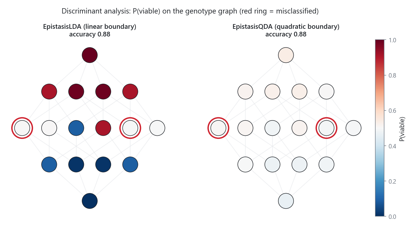
The two differ in the shape of the decision boundary they can draw. LDA assumes a single shared covariance across both classes and produces a linear boundary; QDA fits a separate covariance per class and produces a quadratic one. QDA is the more flexible model but estimates many more parameters, so on small libraries it is less confident (its probabilities sit closer to 0.5) and usually wants regularization via reg_param.

When to use which¶

• LDA when the two classes are roughly linearly separable in the projected feature space, or when data is scarce. Fewer parameters, more stable.
• QDA when you expect the viable and nonviable classes to have genuinely different spreads and a curved boundary, and you have enough genotypes to estimate per-class covariances (regularize with reg_param otherwise).

If you only need a linear boundary with calibrated probabilities, EpistasisLogisticRegression is the simpler choice.

How it works¶

Both models reuse the classifier base procedure:

1. An order-1 EpistasisLinearRegression (model.additive) is fit to the continuous phenotypes to learn each mutation's additive contribution.
2. The design-matrix columns are scaled by those additive coefficients, projecting them onto a per-mutation contribution scale.
3. sklearn's LinearDiscriminantAnalysis / QuadraticDiscriminantAnalysis is fit on the projected matrix using binarized labels (y > threshold -> 1).

Constructor parameters¶

EpistasisLDA¶

threshold (float, required)

Phenotype cut-off. Genotypes with phenotype strictly greater than threshold are class 1 (viable).

model_type (str, default "global")

Design-matrix encoding: "global" (Hadamard) or "local" (biochemical).

solver (str, default "svd")

sklearn LDA solver. "svd" handles collinearity without a covariance inverse; use "lsqr" or "eigen" if you want shrinkage.

shrinkage (str | float | None, default None)

Covariance shrinkage (only with the "lsqr" / "eigen" solvers). "auto" uses the Ledoit-Wolf estimate.

priors (np.ndarray | None, default None)

Optional class priors.

EpistasisQDA¶

threshold, model_type, priors

As above.

reg_param (float, default 0.0)

Regularizes each per-class covariance toward the average eigenvalue. Raise it (for example 0.2) when the projected feature count approaches or exceeds the number of genotypes, which otherwise makes a class covariance singular.

Workflow¶

import numpy as np
from epistasis.models.classifiers import EpistasisLDA, EpistasisQDA

threshold = float(np.median(gpm.phenotypes))

lda = EpistasisLDA(threshold=threshold)
lda.add_gpm(gpm)
lda.fit()

qda = EpistasisQDA(threshold=threshold, reg_param=0.2)
qda.add_gpm(gpm)
qda.fit()

labels = lda.predict()              # 0 / 1 class labels
p_viable = qda.predict_proba()[:, 1]  # P(viable) per genotype
accuracy = lda.score()              # fraction correctly classified

Key methods¶

See also EpistasisLogisticRegression, EpistasisGaussianProcess, and EpistasisGaussianMixture.