`EpistasisGaussianMixture`¶

EpistasisGaussianMixture separates genotypes into viable and nonviable groups with a Gaussian mixture model. Unlike the other classifiers it is unsupervised: sklearn's GaussianMixture clusters the projected genotypes without seeing labels, and EpistasisGaussianMixture then assigns the cluster with the highest mean phenotype to the viable class. The threshold is used only to evaluate accuracy, not to fit.

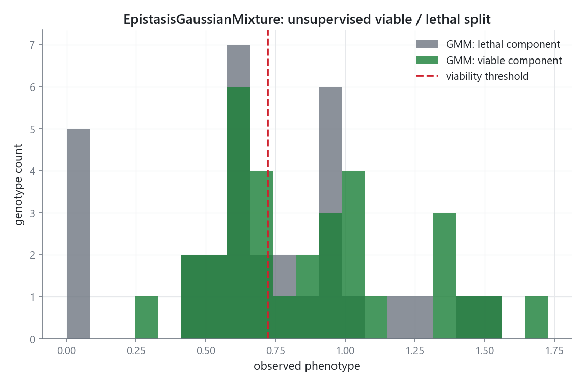
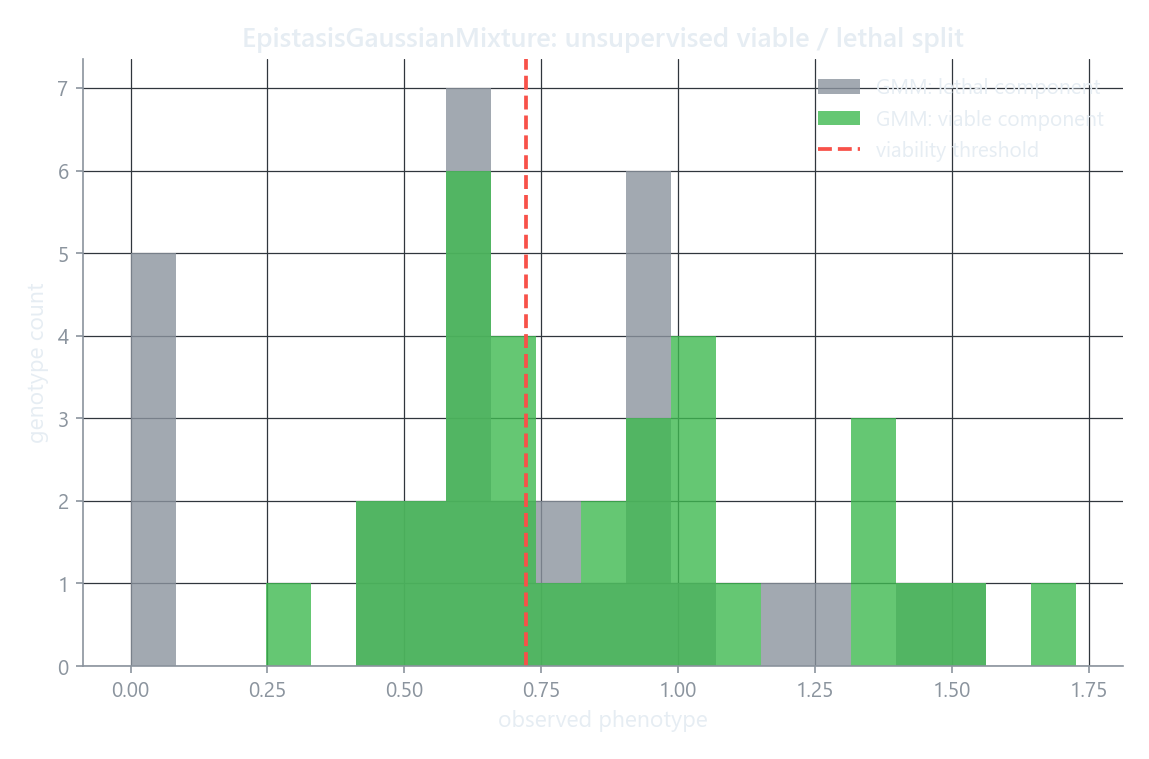
Histogram of observed phenotype with genotypes colored by the mixture component they were assigned to, and the viability threshold marked

The histogram shows the observed phenotypes split by the component each genotype landed in. Because the split is unsupervised, the boundary between components does not have to line up exactly with the threshold (dashed line); the highest-mean component is taken as viable.

When to use this model¶

Use EpistasisGaussianMixture when your data plausibly contains two populations (for example a functional mode and a dead mode) and you would rather discover that structure than impose a hard cut-off. It is also useful as a sanity check: if the unsupervised split agrees with your threshold, the two classes are genuinely separable.

How it works¶

An order-1 EpistasisLinearRegression (model.additive) learns each mutation's additive contribution.
The design-matrix columns are scaled by those additive coefficients.
sklearn's GaussianMixture is fit (unsupervised) on the projected matrix.
The component whose member genotypes have the highest mean phenotype is mapped to class 1 (viable); the rest are class 0.

Constructor parameters¶

threshold (float, required): Phenotype cut-off, used to score accuracy after fitting (not during fitting).
model_type (str, default "global"): Design-matrix encoding: "global" (Hadamard) or "local" (biochemical).
n_components (int, default 2): Number of mixture components. The default of two matches viable / nonviable.
covariance_type (str, default "full"): sklearn covariance form: "full", "tied", "diag", or "spherical". Use "diag" or "spherical" when the projected feature count is large relative to the number of genotypes, where "full" would be singular.
max_iter (int, default 100): Maximum EM iterations.
random_state (int | None, default None): Seed for reproducible EM initialization.

Workflow¶

import numpy as np
from epistasis.models.classifiers import EpistasisGaussianMixture

model = EpistasisGaussianMixture(
    threshold=float(np.median(gpm.phenotypes)),
    n_components=2,
    covariance_type="diag",
    random_state=0,
)
model.add_gpm(gpm)
model.fit()

labels = model.predict()    # 0 / 1, viable = highest-mean component
accuracy = model.score()    # agreement with the threshold labels

Key methods¶

Method	Returns	Description
`fit(X=None, y=None)`	`self`	Fit the additive model then the (unsupervised) mixture, and map the viable component.
`predict(X=None)`	`np.ndarray[int]`	Predicted class labels (0 or 1).
`predict_proba(X=None)`	`np.ndarray[float]`	Class probabilities, shape `(n_genotypes, 2)`.
`score(X=None, y=None)`	`float`	Accuracy against the threshold labels.

EpistasisGaussianMixture¶